Endogeneity And The Marketing Mix Model

Overview

A key focus for most marketing managers is optimal allocation of the marketing budget. This relies heavily on correct causal attribution to each element of the marketing mix. The marketing mix model is a popular method to help inform this process, where ‘nested’ sequences of equations trace out a hypothesized consumer purchase journey, quantifying the impact of marketing investments along the way. This structure is designed predominantly to address the problems of last-touch attribution, helping to reattribute a part of a media such as paid search back to sources earlier in the chain such as TV advertising. In this way, correct credit is allocated to each touch-point leading to improved budget allocation.

However this approach simply assumes a particular causal flow and misses a more fundamental problem. Namely, the inherent selection bias in many online media such as paid search. This creates an endogeneity problem, leading to biased estimates of the search-sales impact in the consumer journey and all marketing effects that work through it. Consequently, even if offline TV advertising does lead to more branded search activity, it does not necessarily mean it drives incremental sales in this way. Without dealing with this problem, budget allocations will continue to be sub-optimal.

The standard mix model

The marketing response model is a popular framework for quantifying financial return on marketing investments, guiding the optimal allocation of resources and sales forecasting. The standard approach takes a simple single-equation form illustrated in equation (1):

$Sales_t =  \sum_{k=1}^K \sum_{l=0}^T\theta_k X_{kt-l} + \sum_{k=1}^K\delta_k D_{kt} + \varepsilon_t$                                                                                                             (1)

where sales (product demand) is specified as a function of a set of marketing variables ($X_t$) covering pricing, promotion and advertising and a set of interventions, seasonal dummies, linear trends and macroeconomic controls ($D_t$). In this model, the left hand side variable ($Sales_t$) is the dependent or endogenous variable and determined 'within' the system. The right hand side variables are the independent or (assumed) exogenous variables and determined 'outside' the system.

The expanded mix model

The emergence of digital marketing has led to path-to-purchase theories where paid, owned and earned media work together to drive demand. This expands the mix model into a multi-equation model or network system, providing a more realistic view of consumer demand and the role of advertising. A simple example is illustrated in Figure 1, comprising natural online search, web traffic clicks (split by source) and product sales.

Figure 1: Network model of short-term sales

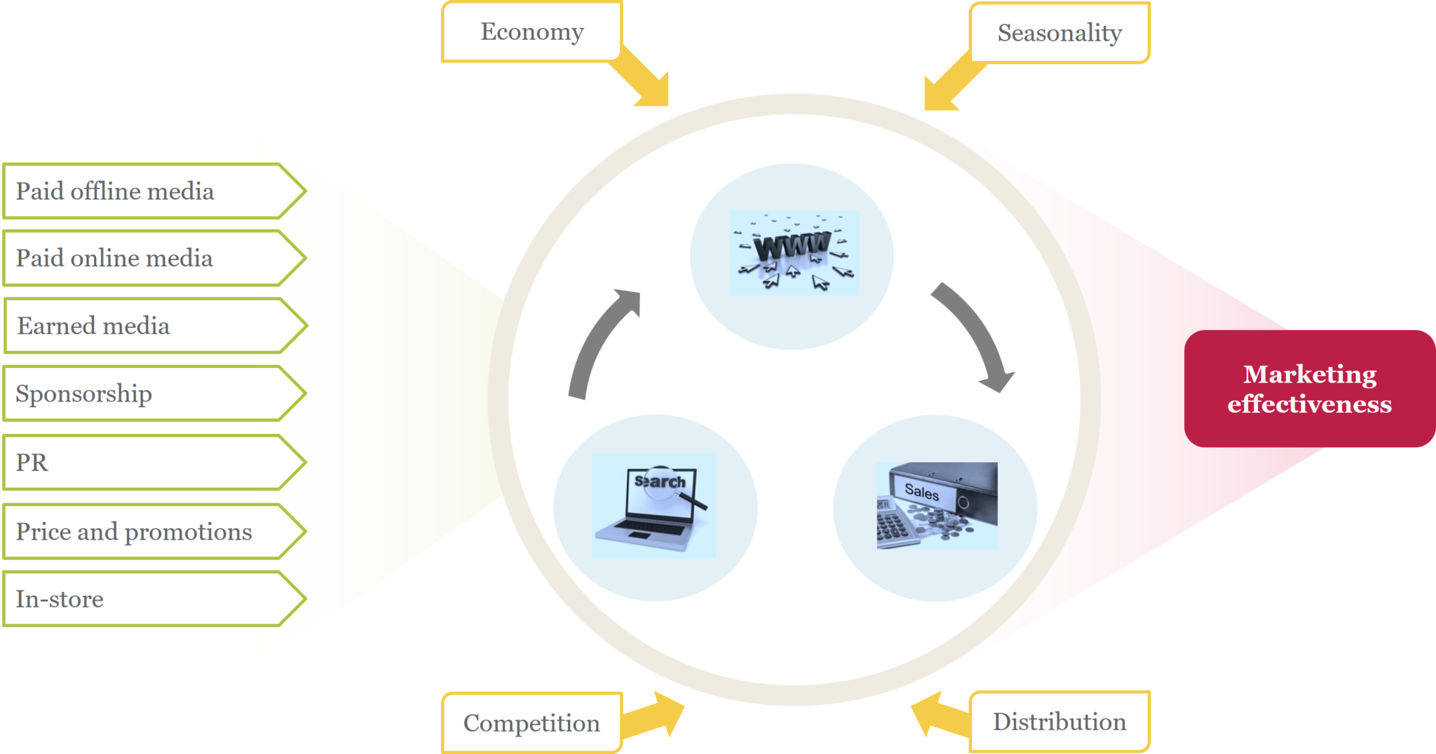
Removing feedback loops, Figure 1 gives six Directed Acyclical Graphs (DAGs) each with a triangular recursive structure and pre-determined causal flow. Commercial marketing mix models typically opt for the type of flow illustrated in equation (2), where marketing variables stimulate a journey from organic online search interest and web site research through to product purchase.

$Sales_t = f(Webtraffic_t, Organic Search_t, X_{kt}, D_{kt})$                                                                                                  2(a)

$Webtraffic_t = f(Organic Search_t,X_{kt}, D_{kt})$                                                                                                                2(b)

$Organic Search_t = f(X_{kt},D_{kt})$                                                                                                                                           2(c)

The endogeneity problem

Equation (2) represents a nested sequence of equations, predominantly designed to deal with last-click attribution bias. However, we now have three endogenous variables: sales, web traffic and natural search. As such, current-period endogenous variables appear as both dependent and independent variables. Endogenous right-hand-side regressors are correlated with the model error term and violate the assumptions of the marketing mix model. This leads to endogeneity bias and poorly estimated model parameters.

The main problem lies in the inherent selection bias in online behaviour.  Selection bias arises when those with the highest propensity to buy may be the most likely to take part in the ‘treatment’ (paid search for example). That is, (part of) the difference in the ‘treatment’ outcome (sales) may be caused by a factor that predicts the likelihood of paid search rather than due to the treatment (search itself). So, consumers with a greater propensity to buy would predict the level of search traffic, which in turn predicts the sales outcome. In this way, a large proportion of site visits are simply an artefact of the sales process.

This creates a simultaneity issue, where sales and web traffic (sources) could equally well be reversed in the chain of model (2). This, in turn, creates a correlation between the endogenous regressor and the model error term. The most serious consequence is a biased estimate of the web traffic-sales impact in equation 2(a) and all off and online marketing effects that work through it.

Solutions

Solving endogeneity bias, in all its forms, is central to correct causal attribution. With observational data, this can only be addressed through established identification techniques to ensure valid causal inference. Here, we consider six key approaches.

Standard panel analysis

The key to causal attribution or inference is the ability to control for confounding factors. As far as the endogeneity of paid search is concerned, the confounding factor is latent purchase pre-disposition amongst consumers. Such unobserved heterogeneity is manifest in correlation between paid search and the error term in an aggregate model. Disaggregated (fixed effects) panel structures for sales can help to deal directly with this, based on the assumption that purchase predisposition is related to characteristics of shoppers across defined cross-sections. Provided this is broadly constant over time and site visits contain little measurement error, fixed effects can eliminate unobserved purchase predisposition from the error term.

Difference in differences

This is a form of fixed effect estimation designed to test the causal impact of interventions in test and control studies. For example, suppose we take two key DMAs and switch off paid search in DMA1 for say 2 months. The difference-in-differences estimate would then compare the 2-month change in sales in DMA1 to the change in sales in DMA2 over the same period. This process amounts to removing the common fixed (base) differences between the DMAs to reveal the causal effect. However, this approach rests heavily on the so-called ‘common trends’ assumption. Namely, that in the absence of treatment (switching off search), the sales of each DMA would have evolved in a parallel way over time.

Instrumental variable estimation

Instrumental variable (IV) estimation is the classic solution to the endogeneity problem, where the causal effect of a variable x on an outcome variable y is estimated using an instrumental variable z which affects y only through its effect on x (the exclusion principle). For example, the causal effect of smoking on poor health could be estimated by using the tax rate for tobacco products as an instrument: the tax rate can only be correlated with health through its effect on smoking. If we find that tobacco taxes and state of health are correlated, this may be viewed as evidence that smoking causes changes in health. 

So it is with paid search: a variable that drives sales only indirectly through search traffic could provide the exogenous variation required to resolve the selection bias problem. On face value, the nested mix model structure of equation (2) appears to fit the bill. Provided (at least one of) the exogenous variables $X_t$ and $D_t$ driving web traffic satisfies the exclusion principle, we could substitute the fitted values from the web traffic equation into the sales equation to give a two-stage least squares (2SLS) estimate of the causal impact of web traffic on sales. However, this is rarely the case, as $X_t$ and $D_t$  generally affect both web traffic and sales. As such, they cannot serve as valid instruments. 

Instrument free approaches

In these approaches, an endogenous regressor such as paid search is split into a latent random variable and a random error. Unique structures are then imposed on/assumed for the latent factor to achieve identification. For example, the latent IV approach assumes a discrete distribution, whereas higher moments and heteroscedastic approaches assume a skewed and heteroscedastic distribution respectively. These assumptions guarantee that the distribution of the endogenous regressor differs from the main model error term. This 'models out' the dependencies and identifies the causal effect of search on sales.

However, these approaches require exogeneity of the latent factor - which is really no different from the exclusion restriction of the classic IV method. More recent incarnations which do not require any exclusion restrictions use copulas to create the joint distribution of the latent factor and the model error term. By directly capturing the correlation in this way, the endogeneity problem is removed. Maximising the likelihood of the joint distribution can then provide the correct model parameters.

Heckman correction

To alleviate selection bias, we need to control for those who are not searching with a truncated regression approach encapsulated in the two-step Heckman estimator. This approach, however, is data intensive, relying on individual observations on the participation decision.

DAG analysis

The simultaneity problem essentially amounts to a focus on just one chain of causality in networks such as model (2), to the exclusion of all others. In DAG analysis, we systematically control for the likelihood of all possible pathways in the consumer journey. By computing the relative likelihoods of all pathways, we may then weight the chosen chain – such as natural search -> paid search-> sales – to help identify the causal impact of paid search on sales. For more details on this approach, see here.